Feature Engineering with Python

Prepping for Algos

Introduction

For starters, here are definitions of feature engineering from different sources. According to Wikipedia, feature engineering uses domain knowledge to extract features(characteristics, properties, attributes) from raw data. According to the book The Data Science Workshop, feature engineering transforms raw variables to create new variables. According to this article, feature engineering uses a technique to create new features from existing data that could help to gain more insight from the existing data.

Features are representations of an aspect of data. For instance, data containing Covid-19 mortality information may have features like age, location, number of deaths, etc.

Why Feature Engineering?

Feature engineering is crucial to building Machine Learning models. Machine Learning is a study of computer algorithms that improve automatically through experience and the use of data. Machine learning algorithms build models based on training data, to make predictions or decisions without being explicitly programmed to do so. Machine learning algorithms are used in a wide variety of applications such as fraud detection, email filtering, cluster analysis, customer segmentation, etc.

Another reason to use feature engineering is to prep your data for a specific machine learning algorithm. If you intend to use a decision tree algorithm, it is intuitive to transform your features in ways the decision tree algorithm will learn.

Data Preparation

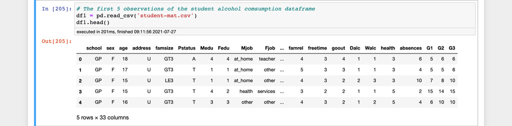
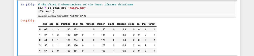
In this article, we will use two datasets to explain feature engineering techniques. The first is a student alcohol consumption dataset hosted on Kaggle and the second is a heart disease dataset hosted on Kaggle

We would use the Pandas data analysis library to perform various feature engineering techniques. The codes will be posted as screenshots but here is the Jupyter Notebook used for this article.

First, we import the Pandas package and the warnings package to silence unnecessary warnings.

Here are the first five observations from the two datasets used in this article.

The student alcohol consumption dataset

The heart disease dataset

Feature Engineering Techniques

Label encoding using the replace() function

The Pandas replace function for label encoding. Label encoding is replacing a categorical variable with numerical values between 0 and the number of classes in the categorical variable minus 1. Label encoding is used for features that have an order of importance also known as ordinal variables.

Let's look at the student alcohol consumption dataset to demonstrate the intuition. The dataset contains a feature named school. The school feature contains abbreviated values representing the name of the schools featured in the dataset. Let's assume the school GP is bigger and better than MS.

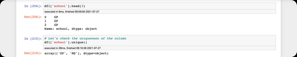
Using the replace function, we replace the categorical values of the school feature with 1 and 2 in the order of importance.

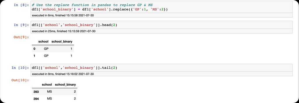
If the schools were greater than two, we would have more than 1 and 2.

One-hot encoding with get_dummies function

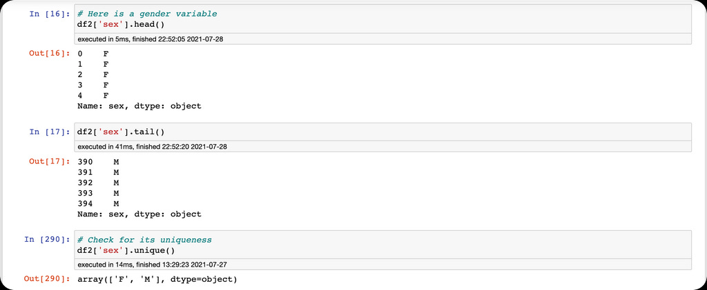
The second feature engineering technique is one-hot encoding using the Pandas get_dummies function. One-hot encoding is a method of converting categorical variables into binary columns. One-hot encoding is used when we want our algorithm to learn that there is no order of importance in the features, also known as nominal variables. Use cases for one-hot encoding include converting variables like male & female, race & ethnicity, etc.

We are going to use the get_dummies function to one-hot encode the sex column into binary columns.

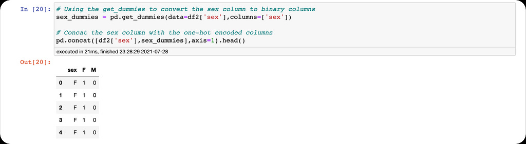
Warning: do not forget to use the drop_first=True argument when encoding to avoid the dummy variable trap.

The qcut() function

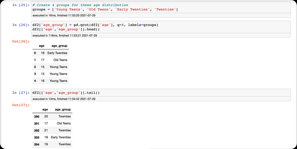
The Pandas qcut() function is used to separate continuous values in a column into four groups. This is often called a discretization technique.

Let's look at the age column in the student's dataset to perform the discretization technique.

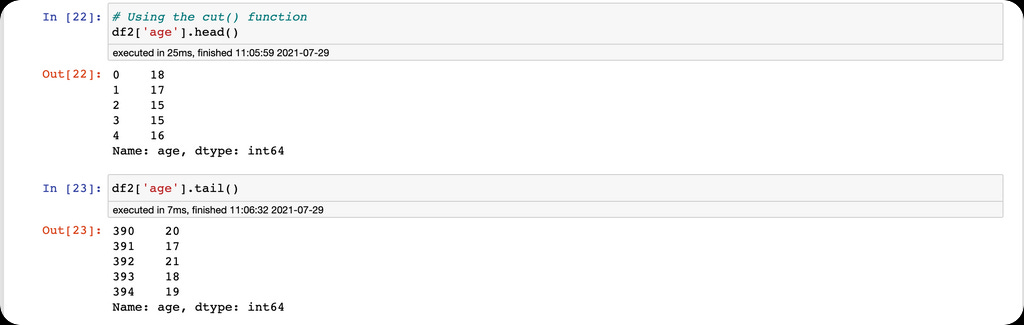
We would take the age values and place them in discrete bins.

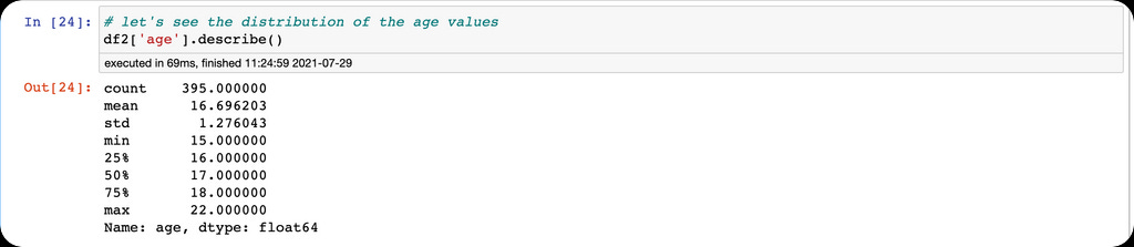
The descriptive statistics show the minimum and maximum values in the age column. This informs our binning intuition. We would create a group with four bins of different age classes, then create a new column with values representing the four bins.

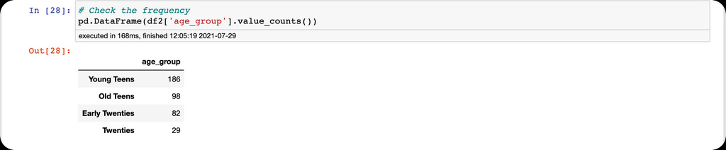
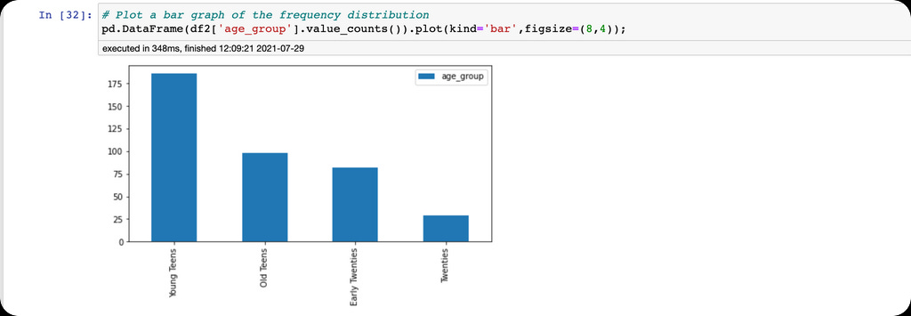
Additionally, we can see the frequency and plot the distribution of the age groups.

Frequency

Frequency Distribution

The cut() function

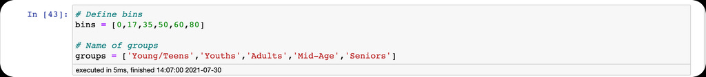
The final feature engineering technique in this article is the Pandas cut function. The cut() function is similar to the qcut() function but with a fundamental tweak. The qcut() function discretizes the continuous variable into four equal bins or quantiles while the cut function doesn't. We just specify the bins and the function makes the split without any guarantees of how the values will be distributed.

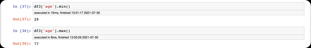
Here, we use the age column in the heart disease dataset to demonstrate the Pandas cut function.

1st & last 5 observations

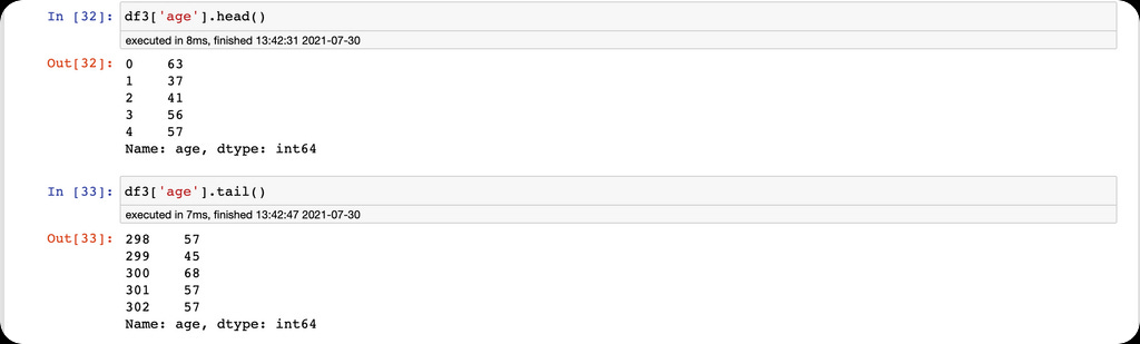
Here we have the minimum and maximum age values in the age column.

Minimum and Maximum age values

We also define a list of bins and groups for the discretization of the age column,

Bins & Groups

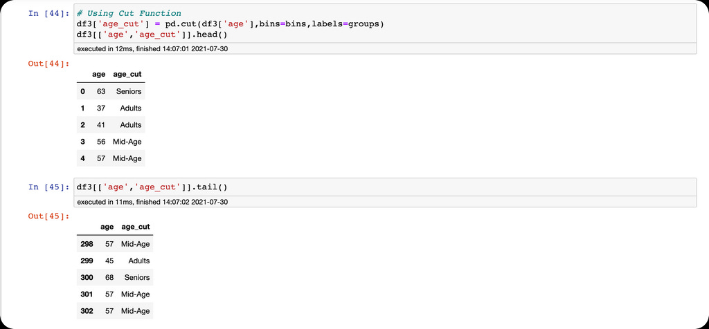
then use the cut function for discretization.

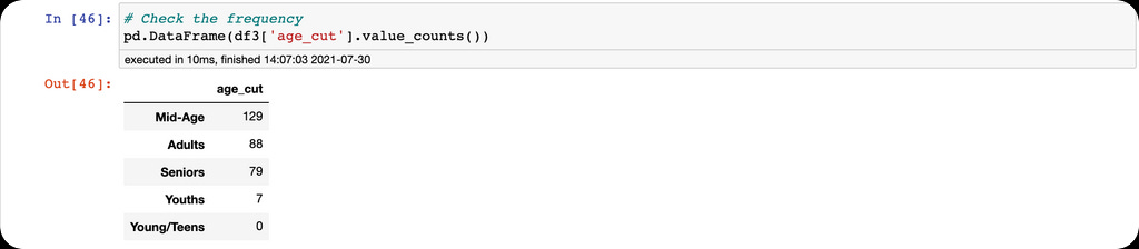
Finally, we count the frequency for each group.

Conclusion

We defined feature engineering as the creation of new features from existing features in a data frame. There are many feature engineering techniques, but we explained label encoding, one-hot encoding, qcut, and the cut function. Feature engineering is a crucial technique for building machine learning models and performing exploratory data analysis.

Reference

1. Feature Engineering using Pandas for Beginners

2. The Data Science Workshop

3. Feature Engineering in Python

4. A Practical Guide to Feature Engineering in Python

5. The Pandas Documentation